Origin of Comets
So where do comets come from? There are two probable sources and for the answer we have to go back in time to before the solar system formed. The primordial solar nebula consisted mainly of hydrogen gas, some helium and a sprinkling of metals distributed from supernova explosions. The nebula began to accrete under the influence of gravity to form a spherical cloud. Continual gravitational attraction resulted in a protostar and potential energy was converted into heat. The protostar eventually became so hot and dense that nuclear fusion commenced in its interior and the protostar became a star. Eventually planets coalesced from the remaining solar nebula and the gas and dust between the planets was swept up.
In 1950, Jan Oort suggested that comets emanate from a vast cloud of material at the edge of the solar system, extending from about 50 000 AU to about 100-200 thousand AU from the Sun. This Oort Cloud, containing perhaps a trillion comet nuclei, is thought to be the remains of the solar nebula which failed to coalesce into the solar system proper. Thus a study of comets enables us to study the materials which comprised the early solar system.
In 1951, Gerard Kuiper proposed a second source of comets. He suggested that a ring of icy material, in the plane of the solar system, must have been left over during formation of the solar system, or ejected by the planets, with its inner edge just outside the orbits of Neptune and Pluto. A similar ring of material has been observed surrounding the star beta Pictoris. For a long time the Kuiper Belt remained only a theory, but in 1992 Jewitt and Luu picked up a 23rd magnitude body 1992 QB1 in a nearly circular orbit at 41 AU (Neptune and Pluto orbit at mean distances of 30 and 40 AU respectively). Since then many more Kuiper Belt Objects have been found.
A comet’s first encounter is probably with Neptune which either ejects it from the solar system or sends it heading for the Sun (in a Neptune crossing orbit). Under the influence of the major planets (principally Jupiter) new comets may have their orbital periods shortened to several thousand years and become long period comets. Further encounters with the major planets may shorten the periods to less than 200 years when they are called short period comets. These comets travel in elliptical, or closed orbits. Most of the short period comets have periods below 10 years. Encke’s comet has a period of 3.3 years and is probably an example of a comet towards the end of its life. It will either disappear altogether or evolve into an asteroid.
Composition and anatomy
We said earlier that comets are probably the remnants of the formation of the solar system. Thus a study of their composition should give us some idea of what the composition was of the primordial solar nebula. So we see that comets contain gases such as hydrogen, ammonia, methane, carbon monoxide, carbon dioxide and water vapour. Smaller amounts of hydrogen cyanide, hydrogen sulphide and formaldehyde are usually present. Apart from these volatile materials we find inorganics, the dust content of comets, typically Si as silicates, Fe, Mg, Ca, Na and other metals. As we shall see later, it is this dust that we observe as meteors, which are nothing more than the debris left behind by the occasional passages of comets around the Sun. So comets contain a complex mixture of frozen ices, gas and dust and this led Fred Whipple to refer to comet nuclei as ‘dirty snowballs’.
Comets consist of three main parts. While far from the Sun where the effects of solar radiation cannot be felt, we have a frozen nucleus, the dirty snowball. The size may vary considerably from comet to comet, but the nucleus of Halley was found to be 16 x 8 x 7 km and rotated every 7.4 days and precessed every 2.2 days.
As the comet nears the Sun, the frozen gases sublimate to form the coma (Latin for hair), with a diameter of 200 000 to 1 million km. The coma is swept away by the effects of the solar wind to form the tail so that the tail points away from the Sun. We classify comet tails into three types:
- A Type I tail (gas or plasma tail) is a straight tail pointing in the direction of the radius vector, due to ionised gases. It is often blue in colour.
- A Type II tail (dust tail) is a plume curving away from the radius vector, due to sunlight reflecting off dust particles. It is often yellow or reddish in colour.
- A Type III tail (anti-tail) is a dust tail seen to extend ahead of the comet. It may be seen when the earth crosses the orbital plane of the comet.
How to observe comets
Different comets appear differently. Some are brighter than others. Some are condensed while others are diffuse. Some develop tails and others not. One or more tails may be visible. The tails may change nightly in appearance. It is up to us as amateur astronomers to document these nightly changes. Let’s look at the format of the observations required.
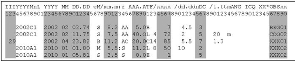
The figure above shows a typical example of a data-set on several comets. ASSA has standardised on the format used in the International Comet Quarterly. If you send me observations in any other format I will convert these to ICQ format before processing. The meanings of the columns are as follows:
Columns 1-3 are reserved for the designation of numbered short period comets. So for example comet Halley is 1P and the observer would enter 1 in column 3. The above example shows an observation of comet 29P Schwassmann-Wachmann.
Columns 4-9 are reserved for the designations of comets observed at only one apparition, with the discovery year in columns 4-7, the half month of discovery in column 8 and column 9 designating the first, second, third comet etc discovered in that half month.
Columns 12-24 give the date in the format yyyy mm dd.dd, in Universal Time to an accuracy of 0.01 days. For example, an observation on 19 November 2006 at 20h45 SAST would give – 2006 11 19, at 18h45 UT and therefore 2006 11 19.78
Column 27, M gives the method used for magnitude estimation:
S = VSS, or In-Out method
B = VBM, or Out-Out method
M = Morris method
Columns 29-32 give the total visual magnitude (m1) of the comet as estimated by the observer. The decimal point appears in column 31. A less than indicator in column 28 indicates the comet was fainter than the magnitude shown. A colon in column 33 indicates the estimate is in doubt or made under adverse conditions.
Columns 34-35 give the reference source used for the comparison stars used to estimate the magnitude
Columns 37-40 give the aperture of the instrument used in cm with the decimal in column 39.
Columns 41-43 give the instrument type and focal ratio with:
L = Newtonian, R = refractor, C = Cassegrain, B = binoculars, E = naked eye
Columns 44-47 give the power used for the observation, flush right with column 47. A naked eye observation is given as 1.
Columns 50-54 are the diameter of the coma, in arc minutes, with the decimal in column 52.
Columns 56-57 give the Degree of Condensation of the Coma, with a value in between integers given as a “/” in column 57. Thus a DC of 5-6 would be recorded as “5/”.
Columns 60-63 give the length of the tail in degrees, or if in minutes of arc a lower case m is given in column 64.
Columns 65-67 give the position angle of the tail in degrees with N=0°, E=90°, S=180°, W=270°
Columns 76-80 give the observers code, usually the accepted ICQ code, or else the first three letters of the surname followed by “xx”. So for example, John Smith would write “SMIxx” until he receives an accepted code.
So you see that the report records details of the time and instrument used and the following details of the comet which characterise its morphology – Magnitude, Coma size and Condensation, Tail length and position angle. Let’s look at how to determine these by observation.
Estimating the magnitude
The magnitude of a comet is estimated in the same way as a variable star, by comparing it against stars of constant, known brightness. The difference is that the comet is rarely star-like and is usually diffuse in appearance. This means we have to do something to compare apples with apples. We achieve this by defocusing the comparison stars to make them approximate a comet in size and/or appearance. It is usual to measure the total magnitude of the coma (designated as m1), but in addition the magnitude of any nucleus or pseudo-nucleus can also be estimated and is designated m2. Only m1 should be reported in the preceding format, m2 should be added in any descriptive notes. The three common methods are as follows:
VSS (Sidgwick) Method (In-Out method) – designated S
The brightness of the in-focus comet is compared with stars which have been defocused until the apparent size is the same diameter as the in-focus coma. The procedure is repeated for several comparison stars to obtain a reliable measurement. It is the comet’s mean surface brightness which is estimated. Thus if the comet shows both a sharp central condensation inside a diffuse coma (i.e a sharp intensity gradient towards the centre), the mean brightness may be difficult to measure accurately. The method is better suited to diffuse comets.
VBM (Bobrovnikof) Method (Out-Out method) – designated B
The star and comet are both defocused by the same amount, until they appear more or less similar in size. When defocused to the same extent the comet usually still appears slightly larger than the comparison stars. The brightness of defocused comet and several defocused stars are compared. The method is better suited to more condensed (DC7-9) comets with sharp intensity gradient.
Morris Method (modified Out method) – designated M
The observer defocuses the comet just enough so that the coma becomes rather uniform in brightness, erasing the generally steep gradient present in most comets from outer coma to central condensation. The comparison stars are defocused separately to the same apparent size as the uniform defocused comet image.
It is important to use accepted magnitude references for the estimation. The SAO magnitudes reference code (S) are generally accepted down to magnitude 9.5. The AAVSO atlas (AA) and AAVSO charts (AC) are handy and reliable references. In the case of AC you should specify which chart was used as a note (eg: S Lupi, d chart). Reference codes are available for dozens of other sources; just check the code with me for that which you are using, but please check the source you are using is considered reliable. There are also a few references which are generally considered unacceptable; the Hubble Guide Star Catalog is one example.
Measuring the coma size
The measurement of coma diameter is an important parameter. Not only does it indicate the comet’s size, but it is also a measure of sky conditions at the time of measurement. Under poor conditions, or when there is haze in the sky, the outer limits of the coma will be lost, leading to an under-estimation of the size of the coma relative to other observers using similar instrumentation. There are three accepted methods of measurement:
- Direct measurement with a micrometer if available
- Estimation of the size relative to two nearby stars of known separation
- Drift measurement – the coma is allowed to drift across the field of view. The length of time in seconds, t, for the coma to drift across a north-south aligned cross-hair is measured. If no cross hair is available then the west edge of the field can be used. The diameter is then calculated from
- diam = 0.25 t cos(dec), where dec is the comet’s declination
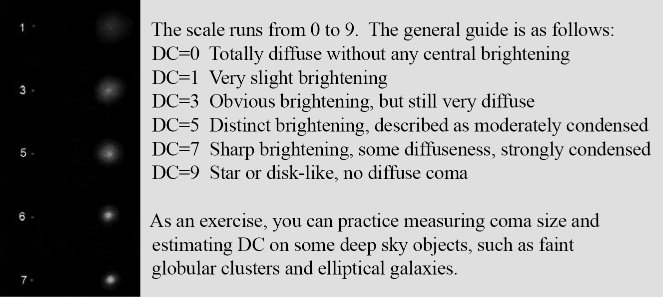
Estimating the degree of condensation
The degree of condensation, which is the existence of a sharp central disk, or sharp brightness gradient intensity within the coma, is simply assessed by comparing the visual appearance in the eyepiece with a pre-drawn scale as shown below.
Measuring the tail length and position angle
Tail length and position angle are best measured photographically. However, accurate visual observations are of use if made in the correct way. The tail is plotted accurately on a suitable star atlas or map. The length is then measured using a suitable accurate ruler, with reference to the scale of the map or by calibrating the measurement against two stars whose separation is known accurately. If the ion and dust tails are both visible then they should be recorded separately. The position angle is simply the orientation of the tail relative to position on the coma or head of the comet from which the tail emanates. It is measured from the plot using a protractor, with celestial north being 0° and east being 90°, etc. Similarly, the position angles of all tails visible should be recorded. If the dust tail is curved, then the length can be measured at various position angles. Remember that the tail length is extremely subjective to haze or twilight, so that attempts should be made to measure the length under as darker skies as circumstances permit.
Sketching the comet
The appearance of the comet can be shown in photos, drawings and CCD images. Much useful work can be done by experienced observers in the field of negative drawings (black on white). Often the human eye will pick up subtle features not visible in photos or with CCDs (jets and hoods in the coma, knots or kings in the tail etc.) and these should be carefully sketched. The final sketch can be used to measure and note the coma size and condensation, length, details and angles of any tails and any other pertinent details along with details of the time, instrument and conditions, to serve as a permanent record for later analysis.
Conclusion
The foregoing is not intended as an advanced treatise in observing comets, but as the essentials required for reliable observation of comets. More details are available from the Director once the observer has mastered these basic skills.
Predictions for comets visible during the year appear in the Sky Guide and updates are available from the Comet, Asteroid & Meteor (CAM) Section.